.svg)


Introduction: When specialization revolutionizes artificial intelligence
In the field of artificial intelligence, a fundamental question arises: how to create models that are both powerful and effective? The answer may well lie in the Mixture of Experts (MoE), a revolutionary architecture that applies the principle of specialization to neural networks.
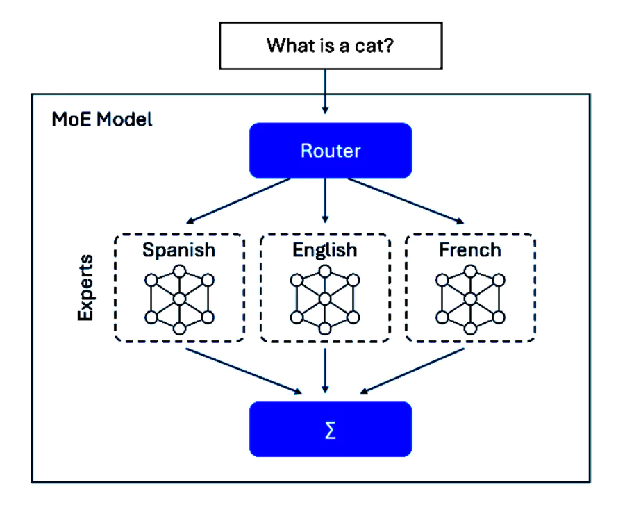
Imagine a company where each employee is an expert in a specific field: accounting, marketing, technical development. Rather than having generalists dealing with all tasks, this organization mobilizes the most relevant expert as needed. That is exactly the principle of MoE : to divide a massive model into specialized sub-networks, called “experts”, which are activated only when their skills are required.
This approach is radically transforming our understanding of large language models (LLMs) and paves the way for a new generation of AI that is more efficient and scalable.
Theoretical foundations: The architecture that is revolutionizing AI
What is the Mixture of Experts in artificial intelligence?
The Mixture of Experts is a machine learning architecture that combines several specialized sub-models, called “experts,” to deal with different aspects of a complex task. Unlike traditional monolithic models where all parameters are enabled for each prediction, MoE only activates a subset of experts depending on the input context.
The fundamental components
1. The Experts

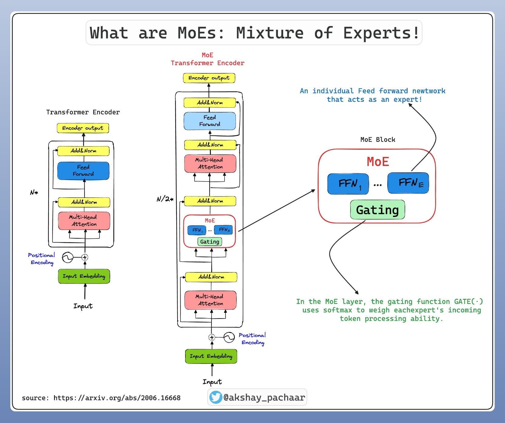
Each expert is a neural network specialized, typically made up of Feed-Forward Networks (FFN) layers. In a Transformer model using MoE, these experts replace traditional FFN layers. A model can contain from 8 to several thousand experts depending on the architecture.
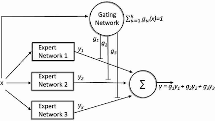
2. The Gating Network
The Gating Network plays the role of conductor. This component determines which experts to activate for each entry token by calculating an activation probability for each expert. The most common mechanism is the Top K Routing, where only the k experts with the highest scores are selected.
3. The Conditional Computation
This technique makes it possible to drastically save resources by activating only a fraction of the total parameters of the model. For example, in a model with 64 experts, only 2 or 4 can be activated simultaneously, significantly reducing calculation costs.
Detailed technical architecture
Entry (tokens)
  ↓
Self-Attention Layer
  ↓
Gating Network → Calculate scores for each expert
  ↓
Top-K Selection → Select the best experts
  ↓
Expert Networks → Parallel processing by selected experts
  ↓
Weighted Combination → Combine outputs according to scores
  ↓
Final release
How it works: Routing mechanisms and specialization
Intelligent routing process

The Gating Network generally uses a softmax function to calculate activation probabilities:
- Score calculation: For each token, the gating network generates a score for each expert
- Top-k selection: Only the k experts with the highest scores are selected
- Normalization: The scores of the selected experts are renormalized to sum to 1
- Parallel processing: The experts selected process the input simultaneously
- Weighted aggregation: The outputs are combined according to their respective scores
Load balancing mechanisms
A major MoE challenge is to prevent some experts from becoming underused while others are overloaded. Several techniques ensure a Load Balancing effective:
Auxiliary Loss Functions
An auxiliary loss function encourages a balanced distribution of traffic between experts:
Loss_auxiliary = α × coefficient_load_balancing × variance_distribution_experts
Noisy Top-K Gating
Adding Gaussian noise to expert scores during training promotes exploration and prevents premature convergence to a subset of experts.
Expert Capacity
Each expert has a maximum capacity of tokens that they can process in batches, forcing a distribution of work.
Emerging specializations
Experts spontaneously develop specializations during training:
- Syntactic experts : Specialized in grammar and structure
- Semantic experts : Focused on meaning and context
- Domain-specific experts : Dedicated to fields such as medicine or finance
- Multilingual experts : Optimized for specific languages
Performance and optimizations

Recent optimization techniques
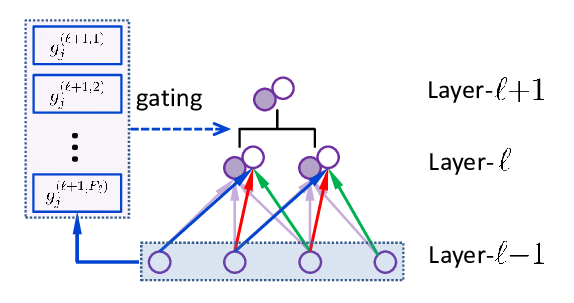
1. Hierarchical Mixtures of Experts
Multi-level architecture where a first gating network routes to groups of experts, then a second level selects the final expert. This approach reduces routing complexity for models with thousands of experts.
2. Expert Dynamic Pruning
Automatic elimination of underperforming experts during training, optimizing the architecture in real time.
3. Adaptive Expert Selection
Learning mechanisms that automatically adjust the number of experts activated according to the complexity of the entry.
Key performance metrics
| 📊 Metric | 🧾 Description | 🎯 Target / Recommended threshold | 💡 Interpretation & Actions (MoE Ops) |
|---|---|---|---|
| 👥 Expert Utilization | Proportion of experts activated at least once in a window (batch / epoch); measures expert coverage. | > 80 % of experts used. | ✅ ≥80 %: healthy coverage. ⚠️ 50–80 %: adjust gate temperature / noise. ❌ <50 %: “dead” experts → increase load-balancing loss or apply expert dropout. |
| ⚖️ Load Balance Loss | Auxiliary loss penalizing variance in activation frequency between experts (importance & load). Value close to 0 = balanced distribution. | < 0.01 (after warm-up). | 🔽 If >0.01: increase loss weight, enable techniques (importance + load), test Similarity-Preserving / Global Balance. Too high hurts quality due to noisy gradients. |
| 🎯 Router Efficiency | Rate of “useful” routings: fraction of tokens whose top-k expert yields expected gain (proxy: router predictive precision / internal F1). | > 95 % (tokens correctly routed). | If <95 %: refine gate (softmax temperature, top-k), reduce noise, distill to a simpler router; monitor collisions (capacity saturation). |
| 🌱 Sparse Activation Ratio | Parameters actually used ÷ total parameters (per token). Indicates operational sparsity. | < 10 % (often 5–15 % depending on k and #experts). | If ratio ↑: reduce k, increase #experts or apply stricter gating; if ratio too low (<3 %) risk of under-training some experts → relax regularization. |
| 📈 Expert Load Variance | Variance (or coefficient of variation) of tokens per expert over a window. | CV < 0.1 (or low normalized variance). | Imbalance → re-initialize gate for inactive experts or enable global load balancing; monitor saturation of few GPUs. |
| 🧮 Capacity Factor Usage | Occupancy rate of expert “slots” (tokens processed / theoretical capacity per step). | 70–95 % (avoid constant 100 %). | <70 %: wasted capacity → increase batch or reduce capacity factor. ≈100 %: risk of rejected / re-routed tokens → increase capacity. |
| 🛑 Dropped Tokens Rate | Percentage of tokens not served by their intended expert (overflow / capacity overflow). | < 0.1 % | If high: raise capacity factor, balance gate, apply expert-choice gating. |
| 🔁 Gate Entropy | Average entropy of gate score distributions (importance). Measures selection diversity. | Stable “medium” range (neither too low nor too high). | Too low → collapse onto few experts; increase noise / temperature. Too high → noisy routing; reduce noise / apply similarity-preserving loss. |
| 🧪 Router Precision (Proxy) | Predictive precision of a supervised model reproducing the gate (audit). Used to estimate routing consistency. | > 70–75 % (observed in Mixtral / OpenMoE) | If low: unstable gate; revisit regularization, check embedding drift. |
| ⏱️ Latency / Token (P50 / P90) | Average and high-percentile decoding time per token. | P90 ≤ 2× P50; stable under load. | P90 explosion → imbalance or network contention (all-to-all); optimize expert placement / parallelism. |
| 🔋 Effective FLOPs / Token | Actual FLOPs consumed vs equivalent dense. | Gain ≥ 40 % vs target dense | Low gain → over-activation (k too large) or excessive communication overhead. |
| 🧠 Specialization Score | Inter-expert divergence of activation / attention distributions. | Divergence > random baseline | Low divergence → redundant experts; apply auxiliary diversity loss or re-initialize inactive experts. |
Practical implementation

Frameworks and tools
1. Hugging Face Transformers
Native support for MoE models with simplified APIs:
from transformers import MixtralForCausalLM, AutoTokenizer
model = MixtralForCauAllm.From_Pretrained (“Mistralai/Mixtral-8x7b-v0.1")
tokenizer = autotokenizer.from_pretrained (“Mistralai/Mixtral-8x7b-v0.1")
2. FairScale vs DeepSpeed
Frameworks specialized in the distributed training of massive MoE models.
3. JAX and Flax
High-performance solutions for the research and development of innovative MoE architectures.
Implementation best practices
1. Initialization of experts
- Various initialization to avoid premature convergence
- Pre-training experts on specific sub-areas
2. Fine-tuning strategies
- Selective gel from experts during fine-tuning
- Adapting routing mechanisms for new domains
3. Monitoring and debugging
- Ongoing monitoring of expert usage
- Routing quality metrics
- Early detection of imbalances
Comparison with alternative architectures
MoE vs Dense Models
| 🧩 Aspect | 🧱 Dense models | 🔀 MoE models (Mixture of Experts) | 💡 Quick explanation / impact |
|---|---|---|---|
| ⚙️ Active parameters / token | 100 % of weights computed every step | ~5–20 % (e.g. top-2 experts out of 8) | 🔽 Fewer FLOPs per token for MoE → higher efficiency & lower cost |
| 🚀 Inference latency | Grows with total size | ≈ latency of a model sized to the “active” set | ⏱️ MoE = quality of a large model at speed of a medium one |
| 📦 Total capacity (parameters) | Must pay for every parameter at runtime | “Dormant” capacity (experts inactive per token) | 🧠 MoE stacks knowledge without a linear inference cost |
| 💾 GPU memory (weights) | All weights loaded & used | All experts loaded, only a fraction computed | 📌 Compute win yes, memory win partial only |
| 🔋 Energy / token | Higher (all multiplications) | –40 to –60 % operations | 🌱 MoE lowers OPEX & carbon footprint at equal quality |
| 📈 Scalability | Diminishing returns (bandwidth, VRAM) | Modular expert addition | 🧗 MoE scales to trillions of “potential” parameters |
| 🎯 Specialization | Single generalist block; global fine-tune | Experts per language / domain | 🪄 MoE improves niches without hurting general tasks |
| 🧭 Routing | Fixed path | Gate picks k experts / token | 🗺️ Dynamic compute allocation based on content |
| 📜 Long context | Cost ∝ size × length | Only active experts billed | 📚 MoE handles very long prompts better |
| 🏁 Parameter efficiency | Performance = active params = cost | Performance > active params | 🎯 MoE ≈ much larger dense (e.g. 12B active ≈ 60–70B dense) |
| 🛠️ Training complexity | Mature pipeline & tooling | Load balancing, “dead” experts | ⚠️ MoE needs monitoring (load balance, entropy gating) |
| 🔄 Updates | Retrain / global LoRA | Add / swap one expert | ♻️ MoE iterates nimbly on new skills |
| 🧩 Client customization | Full fine-tuning expensive | Tuning a few experts | 🏷️ MoE cuts time & cost for multi-tenant personalization |
| 🧪 Robustness / Consistency | Uniform outputs | Inter-expert variability | 🛡️ Requires calibration / distillation to homogenize |
| ⚠️ Specific risks | Cost / energy explode with size | Load imbalance among experts | 📊 Monitor expert-call distribution (load imbalance) |
| 💰 Inference cost (€/1M tokens) | Higher for target quality | –30 to –50 % (depends on k & overhead) | 💹 MoE optimizes cost per quality |
| 🔐 Isolation / multi-tenancy | Hard (shared weights) | Dedicated experts possible | 🪺 Better security / compliance segmentation |
| 🧾 2026 examples | GPT‑4.x, Claude 4, Llama 3.1, Phi‑3 | Mixtral, Grok‑1, DeepSeek V3, Qwen MoE | 🆚 Choice = stable simplicity vs efficient capacity |
| 🎯 Typical use cases | Stable production, consistency needs | Mega-platforms, multi-domain, long prompts | 🧭 Decision: (stability) Dense | (cost + scaling) MoE |
| 📝 Summary | Operational simplicity | Capacity + efficiency | ⚖️ Dense = easy to run / MoE = scalable performance-economy |
MoE vs other sparsity techniques
Structured Pruning
- MoE advantage : Sparsity learned automatically
- Pruning advantage : Simplicity of implementation
Knowledge Distillation
- MoE advantage : Preserving the capabilities of the model
- Distillation advantage : Actual reduction in model size
Ethical challenges

Bias and equity
Experts may develop biases specific to their areas of specialization, requiring particular attention:
- Regular audit emerging specializations
- Debiasing mechanisms At the routing level
- Diversity in the expert training data
Transparency and explainability
Dynamic routing complicates the interpretation of model decisions:
- Detailed logging expert activations
- Visualization tools Routing patterns
- Explainability metrics adapted to MoE
Conclusion: The Future of Distributed AI
The Mixture of Experts represents a fundamental evolution in the architecture of artificial intelligence models. By combining computational efficiency, scalability and automatic specialization, this approach paves the way for a new generation of more powerful and more accessible models.
Key points to remember
- Revolutionary efficiency : The MoE makes it possible to multiply the size of the models by 10 without increasing the costs proportionally
- Emerging specialization : Experts naturally develop specialized skills
- Limitless scalability : The architecture adapts to the growing needs in terms of model sizes
- Various applications : From natural language processing to computer vision
Future perspectives
The evolution of MoE is oriented towards:
- Self-adaptive architectures who change their structure according to the tasks
- Native multimodal integration for more versatile AI systems
- Specialized hardware optimizations to maximize the efficiency of routings
The Mixture of Experts isn't just technical optimization: it's a fundamental reinvention of how we design and deploy artificial intelligence. For researchers, engineers and organizations wishing to remain at the forefront of AI innovation, mastering this technology is becoming essential.
The era of monolithic models is coming to an end. The future belongs to distributed and specialized architectures, where each expert contributes their unique expertise to the collective intelligence of the system.